Error Propagation in Chain Calculations
A statistical look at multi-factor computations. And: Why were inverse and folded scales such important developments?
The general claim about the accuracy of calculations performed using a slide rule with a pair of standard 25-cm logarithmic scales is that it can find answers to about 3 significant digits. In a previous post on the topic of scale length, we talked about how the distance to a number x on a slide rule scale is proportional to the logarithm of that number. So, if a logarithmic scale runs from 1 on the left to 10 on the right, the distance from the left end to a number 1 ≤ x ≤ 10 is given by d = L0 × log x. Here, L0 would be 25 cm for our example.
Using a simple bit of calculus, where the derivative of the natural logarithm ln x is d(ln x)/dx = 1/x, we were able to show that the relative error dx/x in the reading of a number on the scale is proportional to the error in our knowledge of the distance d — call the error Δd — and inversely proportional to the length of the scale, L0:
If Δd is a fraction of a millimeter, say 0.1 mm for instance, and L0 = 250 mm, then Δx/x ≈ 0.001. And for longer L0, the slide rule can be more accurate so long as the thicknesses of the marks on the rule and hairlines used on the cursor are held constant.
But most calculations involve several movements and settings of the slide. If we need to make two or three readings and settings to multiply numbers by adding their logarithms, wouldn’t that make the final answer more prone to error, and hence affect our accuracy estimate? Some such errors might add up, while others might subtract from each other. So what would be an appropriate estimate? And how much do folded and inverse scales help in reducing the number of operations for a multi-factor multiplication or division? I decided to delve a little deeper into this topic to try to understand better the numbers involved in answering such questions.
Number of Steps in a Calculation
A typical 2-factor multiplication calculation using the C and D scales involves the following steps: Align the cursor to the first factor on D; move the slide to align an index on C to the cursor; re-align the cursor to the second number on C; read or interpret the result at the cursor on D. Although this involves a single setting of the slide, it also involves two alignments of the cursor, and a final reading of the answer with respect to the final hairline placement — all sources of error. If the calculation entailed the multiplication of three factors then rather than taking a final reading, in its place we would need to move the slide to align an index at the cursor and then there would be a final movement of the cursor to the third factor on C where the final reading would be made using the cursor — six settings/readings in all. And each additional factor in a multiplication series would result in another setting and another reading.
Note that if we have both multiplications and divisions using only the C/D scales, then one could divide first, and then multiply as this might not require an additional translation of the slide. A three-number computation such as 5 / 2 x 3 = 7.5 can often be found with one setting of the slide and three cursor readings, for example, even though it involves three numbers and not just two. But whenever the slide is moved and aligned using the cursor, when the cursor is moved and aligned with a number on a scale, or when a final value is read using the cursor, there are errors associated with each instance.
Our actual need, of course, is to add or subtract logarithms, which is the addition/subtraction of lengths along the slide rule. To get to our final configuration, we make some number of individual alignments between the two scales. In our example above, moving the cursor to 5 on D and then aligning the 2 on C to the cursor could be thought of a single setting of the slide, since what is important is the alignment of the 2 to the 5, and we are merely using the cursor to facilitate this alignment. But in practice this involves aligning both the number on C and the number on D with the cursor. Just to build up a consistent story, in what follows I will continue to count a setting of the cursor to a number on the rule on the same par as a setting of the slide to the cursor, and count these as individual sources of error.
The Size of the Errors
Whether it is a setting or a reading, the operation involves the placement of a number against the hairline. I have read that a typical hairline is about 0.05-0.10 mm wide (50-100 microns). To best make a precise setting of the hairline to a mark on a slide rule scale, the marks should be slightly wider than the hairline, as we shall see below. To examine this a bit further, I took out my trusty Frederick Post Versalog II slide rule — a high-quality Japanese-made bamboo slide rule — and attempted a couple of measurements. I took a photograph that contained the hairline of the cursor as well as the L scale. The L scale runs linearly from 0 to 1 and, on the Versalog at least, has 500 divisions. Since the complete scale is 25 cm = 250 mm long, then there is 0.5 mm/division.
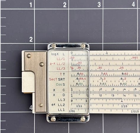
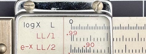

To get an idea of line widths, I used a “Powerpoint”-style program to make lines on the image and read off their lengths, using the default unit on the screen of “points”. Finding 43 pts as a typical value for the distance between lines on the L scale, I found that the lines on the slide rule appeared to be about 12 pts wide; scaling, this corresponds to 12/43 × 0.5 = 0.14 mm in width. And the cursor hairline is about 8/43 × 0.5 = 0.093 mm in width. Thus the scale lines are about 50% wider than the hairline.
None of this was done very scientifically; issues such as shadowing, parallax, and so on could easily affect my interpretation of the line widths using this technique. But it does set the scale. So to ease our attempts in future estimates, let’s just assume a hairline is 100 microns wide, and the marks on the rule are 150 microns wide. We can always scale our answers later if necessary.
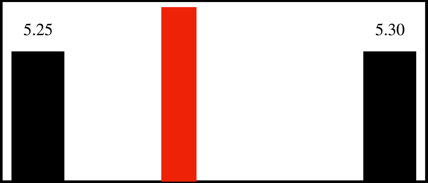
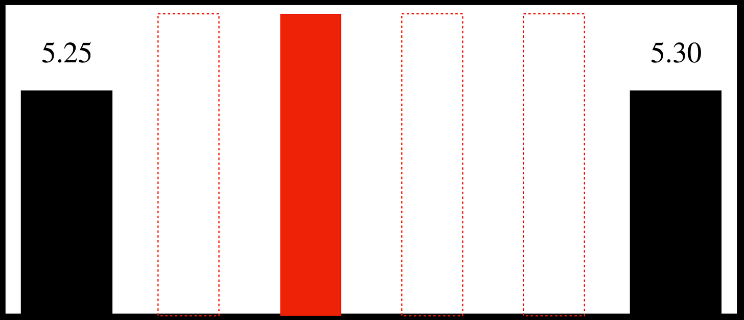
So, would the 100 microns of our cursor hairline be our setting/reading error? The human brain is amazing when it comes to visual comparisons. In the images below, the black rectangles are 150 units wide, and the red rectangles are 100 units wide. The left-most pair has the centers of the two perfectly aligned. In the next set, the “cursor” is off-centered by 5 units (read as 5 microns) and is already fairly discernible. Of course, this image is highly “magnified” compared to what one would see on a slide rule without the use of magnification. But by the time we are off by around 10 microns, it is pretty easy to see even from a distance. For reference, our eyes and brains are good at comparing the size of the black area on the left to the black area on the right. In order, the ratios of right area to left area in the images below are: R/L = 1, 1.5, 2, 3, and 4. After playing around with it, I came to believe that a very careful alignment of the cursor to a mark on the slide rule can be accomplished to within ±10 microns on a high-quality slide rule such as the Versalog.
So with such line thicknesses, the placement of the hairline against the left or right index on the slide for instance would be very precise. But for numbers in general, this precision might only occur if the number had just 1 or 2 digits, perhaps 3 digits on the left-end of the rule. Getting that third or sometimes fourth digit might take some interpolation between marks on the rule, and so the error in the setting/reading will also depend upon the skill of the user.
Suppose we want the cursor to line up against the value 5.27 on the D scale of a 25-cm slide rule, just taking a point at random. Most such rules might have marks at 5.2 and 5.3, and likely a mark at 5.25. The “7” would need to be interpolated by the user. On a 25-cm slide rule, the distance between 5.25 and 5.30 should be
and the location of “7” would be roughly 0.4 mm to the right of the “5.25” mark. The eye can separate the space between 5.25 and 5.30 into two relatively equal regions, and so setting “5.275” is not very hard. Setting 5.27 would just be a little to the left of center. Using our same rectangles as before, here is the cursor set at 5.27:
One might also imagine four “spaces” between the two black marks and placing the cursor in the second “space”. This is generally not too difficult, since the space on the right of the cursor is roughly twice that on the left (perhaps a tad less):
So for this particular example, I can imagine setting the cursor with an error of about 0.0025 (i.e., perhaps placed at 5.2675 as opposed to 5.27) which is equivalent to being off by a distance of 250 mm × (log 5.27 - log 5.2675) = 0.05 mm, or half of a hairline thickness; perhaps this is a bit of an overachievement, but I think that with practice such settings can be routinely achieved.
You might say to yourself that setting a number like 9.77 on the slide rule is much harder to achieve, but
is still 5 hairline thicknesses and so a pretty good setting can still be made. And even if the third digit is off by 1 (9.76 instead of 9.77, say), this is still about 1 out of 1000 for this single-number setting.
From these arguments the overall accuracy of a setting or reading on a good-quality slide rule can be in the range of 10’s of microns. In our following examples I will use 50 microns (0.05 mm).
A setting error of 0.05 mm on a 25-cm slide rule C/D scale gives a relative error on our selection of “x” of about 0.0005, through our arguments at the beginning of this post. But we also said that we would need to make 4 settings or readings using the cursor in a multiplication or division of just two numbers. The errors of these 4 settings will then “add up” into a single overall error in our result. But they won’t all be 50 microns, and they won’t always add up to 0.2 mm. Sometimes the cursor setting will be off to the left, sometimes to the right, sometimes bigger and sometimes smaller.
If a calculation were to be repeated, the individual errors introduced in our second attempt are likely to be very slightly different than the errors made in the first attempt, and hence the two results we obtained for the same calculation will themselves be slightly different. So when speaking of “a typical error”, if we imagine repeating a reading or a setting over and over again, then there will be a spread in our results, according to the usual Normal (“bell-shaped”) distribution.
Which brings us to our standard statistical analysis.
The rms Error
When speaking of a “typical” error I, at least, think of the “rms” (root-mean-square) of a distribution that has been built up over the course of many such reading and setting operations. Suppose we repeat a calculation P times in an attempt to determine a final value of a variable that we’ll call D. To emphasize the point, in the images below I have selected ten thousand numbers (P = 10000) from a Normal distribution using a random number generator that produces an average of ⟨D⟩ = 1000 and a root-mean-square Drms = 1. If I make a histogram (shown below) of the 10000 numbers that were selected, we see the typical bell-shaped distribution, and we find the computed mean and rms for this trial are 1000.013 and 0.9989, respectively, via computer.
As a reminder, the root-mean-square, xrms, of a variable x is given by
For a distribution with a mean of zero (⟨x⟩ = 0), the rms is simply
Now if I only take the first 1000 values from my random sample, I still get an rms of about 1. If I take the first 100 or even the first 50, I get an rms of about 0.9. And if I take the first 10 numbers, or even just the first 4 numbers, I find rms values of this same general magnitude.
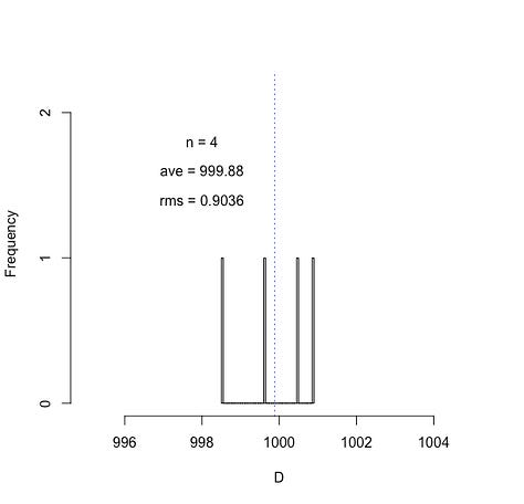
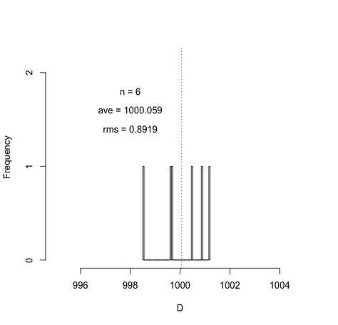
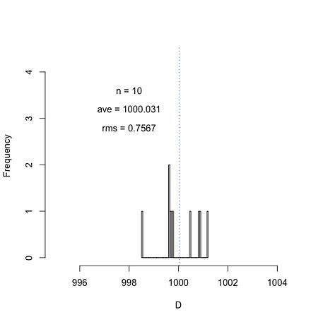
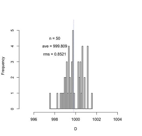
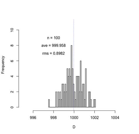
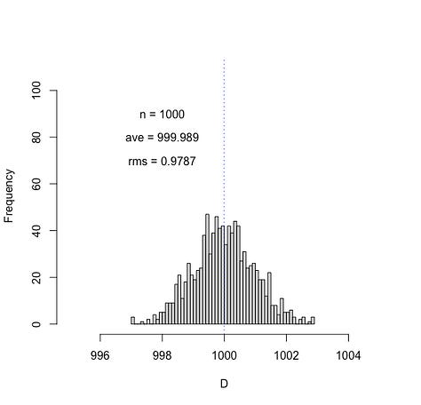
Of course the above plots are for one particular running of the random number generator. Another “roll of the dice” would give different numbers and the plots for small “n” values will no doubt look different. But in the long run over thousands of numbers picked, about 64% of the time the randomly drawn value D will be within 1 of the expected average value of 1000.
A slight aside: Small n vs. Large n
A glance at the histograms above can easily give the impression that the rms is fairly insensitive to the number of samples drawn from our distribution of settings/readings. But this was actually a fairly lucky (though, not atypical) draw of the numbers. It is not hard, for example, to imagine drawing 4 numbers that could create a much different average and much different spread about that average than what is shown above. To illustrate, suppose we have our same settings of the random number generator, but choose a different set of n random numbers each time. For instance, suppose we take four numbers from our set and find their average and their rms about that average. And next, repeat this process P times. For P = 1000, we get the following results:
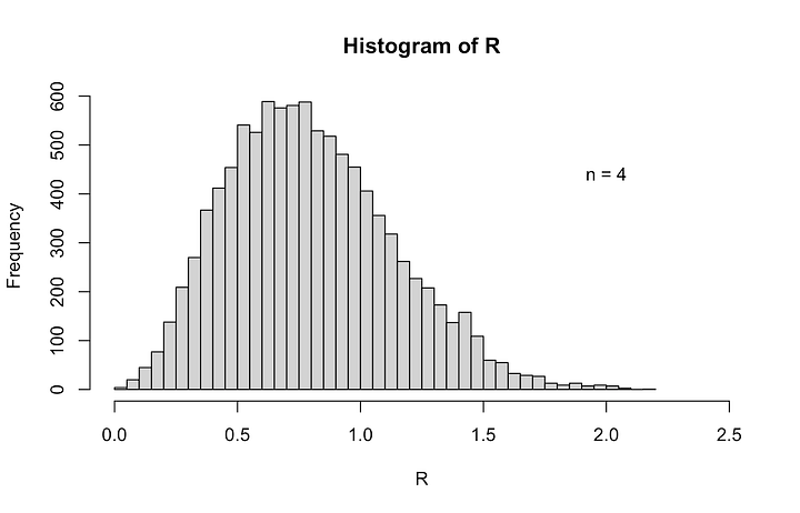
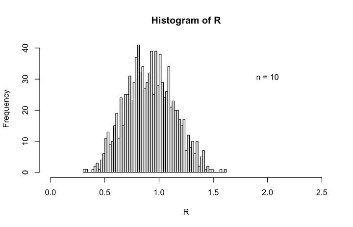
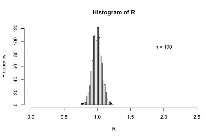
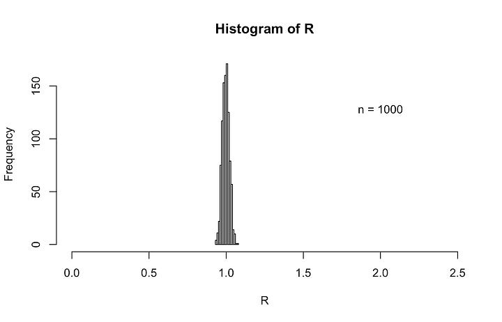
We see that the rms values that are computed for 4 random numbers has a large spread around the expected rms of 1, and peaks slightly below 1. But if we look at larger sample sizes, such as for n = 100 or 1000 — in fact, even for n = 10 — the computed rms values will converge toward the expected number of 1 and the spread around that value gets increasingly narrow for larger n.
The effect at small sample size can be adjusted for by a correction first introduced by Frederick Bessel (of Bessel Function fame) in the 1800s and is named in his honor. It involves re-writing the expression for rms — often called the Standard Deviation — as
to give a better estimate of the true rms of a distribution when the sample from the distribution only consists of a small number of observations. In our earlier example of n = 4, we found an rms of 0.09. But the “true” rms for larger sample sizes can be better estimated as √(4/3) = 1.15 times this, which for our earlier example happens to yield about 1.0.
But I digress…
Analysis of a Calculation
OK, so now let’s apply what we’ve been talking about to the case of a slide rule calculation. Several movements of the slide or cursor are performed in a chain calculation, which facilitate the addition and subtraction of the logarithms of the numbers involved. Again, imagine for now that we are just using the C and D scales for performing multiplications and divisions. And imagine that the slide rule begins with the indices on C and D perfectly aligned with each other. Now when several factors are involved, including both multiplication and division, there are many ways to arrive at a final answer. But we must end up with the slide in a certain position where the final answer will be below the hairline of the cursor on the D scale.
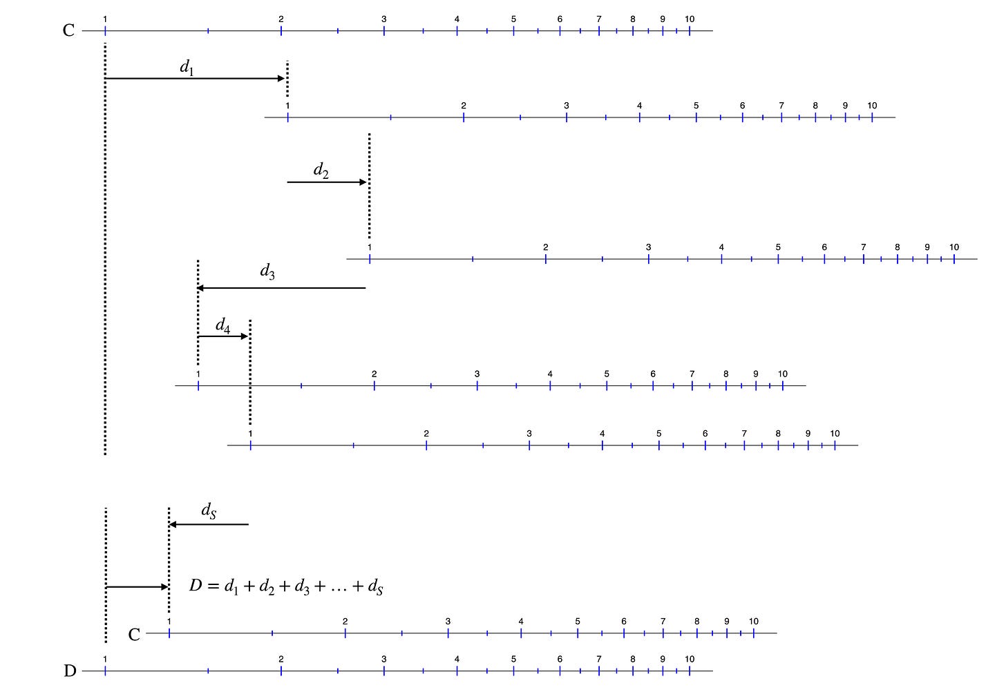
Suppose that the final displacement, D, of the slide (initially, D = 0) with respect to the left end of the stock is the sum of displacements labeled di as shown here, created through S such movements:
The ideal final displacement D at the end of the calculation is
The various di values, where 1 ≤ i ≤ S, are the ideal displacements for the intended calculation and will be positive or negative, depending on the movement of the slide to the right or left when adding or subtracting logarithms. The final displacement D is guaranteed to give us the correct answer directly below the final (ideal) setting of the cursor.
But moving the slide and aligning it with the stock using the cursor results in more than just S individual errors. From our earlier discussion it is apparent that a single setting of the slide can have in itself the build up of errors from a previous setting of the cursor. For example, to make a new slide setting, we move the cursor to be at a factor on C. This introduces an error on the setting of the cursor. So even if we now moved our slide index to a perfect alignment with the cursor, it’s still in the wrong place because the cursor is in the wrong place. And since the alignment of the index to the cursor is imperfect, we have two errors in this process — the error in the initial placement of the cursor, and the error in the placement of the slide with respect to the cursor. Hence, while there are S moves of the slide in a calculation, there are actually more than S errors that contribute to the final answer. In general, there will be some total number of errors N, due to the setting of the cursor, where N > S. If we were performing only multiplications using the C/D scales, for instance, we would have N = 2S + 2.
The actual final displacement of the slide will be given by D + ΔD, where D is the ideal position of the slide to yield the true final answer. The final placement error, ΔD, will be the sum of all of the individual reading/placement errors Δdi
due to both cursor-to-number and number-to-cursor operations. Since the values of the errors Δdi are random and assumed from a Normal distribution, and can be positive or negative, then there can be some amount of cancellation that goes on.
So now imagine performing a particular calculation on the slide rule which has N steps. If we repeat the calculation — step for step — it is very possible (probable) that the error at each step will be slightly different than the time before. So, to get a “typical accuracy” for a multi-step chain calculation, we look at the expected rms deviation for an N-step calculation if we were to repeat that calculation a large number of times, P.
For each of the P attempts, the ideal final slide position D would be the same. But, we would arrive at a different total ΔD for each case due to the different errors introduced for each trial calculation:
The Δd values in this list are all different. That is Δd11, Δd21, …, Δd12, Δd22, …, Δd1P, ΔdNP are all randomly chosen from a bell-shaped error distribution. There would be N×P values in all. We expect our distribution of errors Δd to have a mean of zero, and an rms spread, Δdrms. Since Δd has a mean of zero, then on average ΔD will as well. This only tells us that if we perform the same calculation a large number of times (large P), then the average of the slide positions of these attempts should be very close to the ideal final setting D.
Next, we estimate the value of ΔDrms — the spread in the final displacement from all of our repeated calculations. The rms of our ΔD distribution is given by
since the average ΔD is zero. But this large sum turns messy in a hurry, since each ΔDi has N terms. We would need to square each of these ΔD’s — hence creating N2 cross terms — and sum all of these sums (there are P of them) and then divide by P. So, to keep track of this operation, we write the above summations of all of these terms in the following form:
Though the values of Δd are all randomly chosen, there are terms in this grand sum where i and j have the same value. When this happens, Δdik × Δdjk = Δdik2 is a positive number. Otherwise, for i ≠ j, the Δdik × Δdjk values will be random, including their sign. So for a large sum, the strictly positive values will add up to a large number, while the addition of the terms with random plus-or-minus values will tend toward zero, or at least their sum will be insignificant compared to the sum of the P values that must always be positive. Hence, we get the following:
In the above notation, 𝒪(0) refers to a “term of order zero”, meaning it is insignificant compared to the first term, and so will be ignored. Again, the symbols “⟨x⟩” refer to the average of the variable x. Since all of the errors Δd are from the same distribution (Normal, with zero mean and the same rms), then when averaged over our large number P,
which was used in the last step. And so, what we find is that
This says that if we can set/read the slide/cursor with a typical error of Δdrms, then the typical error ΔDrms in the final placement of the slide/cursor after N settings -- representing the final answer -- will be larger than Δdrms by a factor of √N.
We have just performed the famous “random walk” calculation for a Normal distribution.
The Final Result
We started this discussion by remembering that the error in making a setting to x on the slide rule depends upon the error Δd in reading/setting the appropriate mark on the rule and is given by
A final result of a calculation that requires N settings of the slide or readings of the cursor will result in N errors caused by the ability of the user to set the cursor to the right location, and by the physical line thicknesses, and so on. Thus, the final location of the cursor on the D scale, say, will be the true desired location D plus our final error value ΔD. While we won’t know the exact value of ΔD we can say that it typically should be within a range of values that are about ±ΔDrms from the true location being sought.
But now, after all that work we did above, we can state that a good approximation for the typical (rms) numerical error for the result of a calculation requiring N settings of the slide or readings of the cursor can be characterized by:
Suppose Δdrms = 0.05 mm, and L = 250 mm; ln 10 = 2.30.
For a single reading of a number under the cursor we can expect
Δxrms/x = 2.3 × 0.05/250 = 0.12/250 ≈ 0.5/1000.
For a 2-number calculation we can assume N = 4. Then the error would be twice the above (√4), or
Δxrms/x = 2.3 × 2 × 0.05/250 ≈ 1/1000.
Suppose N = 16 (about an 8-number chain calculation); then,
Δxrms/x = 2.3 × 4 × 0.05/250 = 9 × 0.2/1000 ≈ 2/1000.
Even for N = 40 (about a 20-number chain calculation); then,
Δxrms/x = 2.3 × 6.5 × 0.05/250 = 14.5 × 0.2/1000 ≈ 3/1000.
I can imagine (but won’t do it) carefully doing a 20-factor multiplication and division problem and getting an answer of 35400 where the true answer is 35312 and being very happy with that result. (0.3% of 35312 is about 100.)
If the rms error were 0.1 mm — or if a 5-inch slide rule is used, for instance — then these numbers would double. And, of course, if we have a 50 cm = 500 mm slide rule, these error estimates are cut in half.
Separation of Errors
In addition, as we noted up front, the error in setting the cursor to a line on the rule is likely a bit less than the error in setting the cursor with a general number, which might need some interpolation between lines. So, one could divide our result for N sources of error into two parts, where one part contains Ni errors from setting the index to the cursor, and the other part contains Nn errors from setting the cursor with a general number; and we’d have N = Ni + Nn. We now could assume settings of the cursor to index have rms error Δdi (say, 10 microns), and settings of the cursor to a general number have rms error Δdn (say, 50 microns). Doing so, we arrive at an equation of the form
Note that for the estimates we’ve been using, the factor (Δdi/Δdn)2 = 1/25. If the numbers Nn and Ni were roughly equal, then the second term under the radical above is only about 4% the value of the first term. This means our previous factors of √N would be replaced by √Nn ≈ √(N/2) , or a reduction of the general overall error in results by about 30%. (√(1/2) = 0.707.)
For our previous example using N = 40 (about a 20-number chain calculation) we had
Δxrms/x = 2.3 × 6.5 × 0.05/250 = 14.5 × 0.2/1000 ≈ 3/1000.
So if we can set the index with the cursor and vice versa with 10 micron accuracy, this would create a revision in our estimate to Δxrms/x ≈ 2/1000 — a nice improvement, but perhaps not a game-changer. It just emphasizes further the level of the overall performance of a standard high-quality slide rule.
I began thinking about this topic as I was exploring the development of new scales at the turn of the 19th century, such as the introduction of the CI and folded scales onto mainstream slide rules. At first I was expecting to find that special scales such as CI, CF/DF, and CIF, were provided to improve accuracy through the reduction of steps in a calculation, and the reduction of needing to reset the index. For example, multiplying three numbers with only C/D scales takes N = 6 steps, with 2 movements of the slide. Including folded and/or inverse scales in the calculation allows one to move the slide only once, but still involves N = 4 steps. This reduces the expected error by only a factor of √(4/6) = 0.816, or by 18%. A 5-factor multiplication that takes N = 10 steps to complete using C/D only, can be done using the full scale set with inverse and folded scales in only N = 6 steps, for example. If the overall error scaled with N, then this would reduce the error by about 40%. But scaling by √N means reduction in the estimated error by only a factor of √(6/10) = 0.77, or a 23% reduction.
And if we suggest that setting errors between the cursor and index is much better than setting errors between the cursor and a general number, the improvement is on the level of a few 10s of percent.
What I have come to appreciate is that the accuracy of the standard slide rule is already very good, particularly for a practiced veteran of its use. (Not me, by the way.) The real advantage of the special scales like inverted scales and folded scales, I would say, is the time savings. More important than getting that extra digit in the answer might have been getting the answer before your competition did! Or, perhaps to quickly return those stranded astronauts back to earth. Or, perhaps, just to meet that Monday morning deadline. It’s the time savings created by (a) not having to perform as many movements of the slide and cursor, but also (b) not having to move the slide long distances and then perhaps finding the need to reset its index. With the folded and inverse scales computations could be performed much more quickly. In the exploration of engineering options in a large project, or for making business decisions, many computations would be performed and time was of the essence for making rapid progress.
With care, when performing a computation with 4-5 numbers or so, the result is still going to be good to 3 digits in the end (typically) — and even for 5-10 numbers results are still in this realm. This is all due to the high-quality slide rules created in the 1900s with their engine-divided scales, and due to Mannheim’s invention of the cursor, especially one with a very thin hairline.
In summary, the final Δxrms/x expression presented is the “rms” of a distribution of a repeated evaluation of a single calculation. It represents the “spread” of a bell-shaped distribution of a large set of evaluations. While a single, particular evaluation could be off by more than this amount (or, perhaps even less) our estimate is indicative of the typical accuracy to be expected.
So, when in doubt — repeat! And with the practice obtained through this repetition, you might actually improve your interpolations of numbers between the lines on the slide rule scales.
Postscript: By the way, my favorite resource for how to efficiently compute using a modern slide rule with the “DF [ CF CIF CI C ] D” scale set (as well as providing great advice for many other scales) is the book entitled, The Slide Rule, by Lee H. Johnson, D. Van Nostrand Company, New York (1949). It is one of the better written and most thorough examinations of computational procedures using the modern Duplex slide rule such as the Versalog, the Deci-Lon, and so on. If you want to learn to make rapid computations, this book is a must-read.



A terrific explanation of the error in slide rule settings, backed up by a great piece of mathematical work. That's a lot of work and energy put into it. Great stuff.
I initially learned to use a slide rule with a basic Pickett and K&E manual. When looking for more information, I came across the book by Lee H. Johnson. It is a terrific resource and I have learned to become much more efficient in my calculations through his methods. Chain calculations used to be difficult and I would lose my place. Not anymore. I refer to it often.
As for interpolation a hairline position, I seem to be blessed with a very sensitive resolution of small offsets. Even when I was a kid, my parents said I had calibrated eyeballs. Even now, I can discern 1/4 inch in 10 feet out of level very readily. Maybe just lucky!?
Terrific piece of work. Thanks.
Awesome stuff Mike. A bit of a surprise at the end - the folded and inverse scales do help improve accuracy, but perhaps not by as much as might be expected.
I agree with your recommendation of Lee Johnson's book and his center-drift method of doing calculations with the folded and inverse scales. It definitely helped me become more proficient with basic slide rule calculations.