
Returning Full Circle
Navigating our way through the world of slide rule history these past few months has brought us from Mercator maps to evaluating hyperbolic functions and back.
Over the past several months we have had a number of articles related to the historical development of the slide rule and its scales. After discussing the sector, and the addition of values from trig tables to perform a multiplication, we turned to Napier’s logarithms and their almost immediate placement upon Gunter’s rules to ease in everyday multiplication and division. It was pointed out at that time how other scales on Gunter’s rule were related to reading and computing navigational parameters, particularly for use on a map with Mercator projection. This was discussed further in an even earlier post on the topic of a Rhumb Line Computer, where we also talked a bit about the Gunter’s special scales for navigation.
After a review of early developments, such as gauging rules, Carpenter’s rules, and Engineer’s rules, we found that the Mannheim slide rule scale layout, along with its cursor, helped to accelerate the development of the modern slide rule. With other scales soon added to slide rules, facilitated often by the cursor, we were eventually led to discussing Vector slide rules. With scales for involving hyperbolic trigonometric functions as their main feature, these rules were first implemented in the late 1920s, and included slide rules that could evaluate hyperbolics through the use of the Gudermannian function, which was introduced to the world in the early 1800s.
During my investigations into Napier, and his strong interest in the easing of calculations used in maritime navigation, I had read that the equation of a Great Circle when plotted on a Mercator map projection involved hyperbolic functions. I knew this made sense, as the Mercator projection and Gudermann’s function were related. In fact, cartography — particularly the Mercator projection — was the origin of the study of the Gudermannian and inverse Gudermannian functions.
And a couple of weeks ago or so I realized that we have discussed all the tools we need in order to go through this final connection – including the right slide rules!
Related previous posts:
Trig Tables – use of trig to perform basic multiplication/division
The Sector – basic tric, calcs, etc.
Napier’s Model – the early development of logarithms
Gunter’s Rule – Line of Numbers, Rhumb, Mer, and other scales
A Rhumb Line Calculator – the Mercator map
The Hemmi 153 – Gudermann’s function
From the early development of logarithms for navigation, to the Hemmi development of their Vector slide rule, we’ve gone somewhat “full circle” in our navigational story. We have discussed rhumb lines and Mercator maps in some detail, but we still should talk about the Great Circle to finally connect everything. So let’s just fill in a few remaining gaps.
A Clergyman, a Cartographer, and a Mathematician Walk Into a Bar…
Gunter, Mercator, and Napier stop into an establishment for a late-afternoon refreshment. There’s plenty of table space up front, but hardly anything near the bar in the back, which was obviously where all the action was. Mercator yells above the noise, “We need to get to the bar before anyone else comes in, so we need to get there as fast as possible!”
Mercator starts creating a map of the environment using his special coordinates. And soon, with his new map in hand, he begins to plan a rhumb line for the journey. But, scratching his head, he quickly admits to his colleagues that this would not be the shortest route of all. “What we need is a quick calculation of the Great Circle!” he exclaims. So he and Gunter discuss strategies while Napier stands quietly by.
Gunter pulls out his trusty sector and starts measuring angles and creating ratios of trigonometric functions, but gets quite nervous when a new group of sailors starts to come through the door behind them. “Oh Gerardus,” he exclaims, “If I only had better scales on this sector of mine…”
Gunter and Mercator look at each other, and then both turn slowly to look at Napier. Says Edmund, “My goodness, John, you’ve been awfully quiet through all of this. Don’t you have anything to add?”
With my strong apologies for the above, let’s reminisce about the development of the Mercator map and its importance in navigation.
To navigate from one place on the globe to another, particularly across oceans where there are no identifying landmarks to view, the great map maker Gerardus Mercator created a map projection, first made famous as a map of the world in 1569, that would allow one to draw a straight line from one point on the map to another, and from the slope of that line compute a compass bearing that would join the two. The course itself is not a straight line, naturally, but all “lines” on this particular type of map correspond to constant course bearings due to the map’s projection properties.
A compass bearing is basically a constant angle relative to a north-south meridian. Since circles of constant latitude on the globe vary in radius according to 𝜌 = 𝑅cos𝜃, where 𝑅 is the radius of the Earth and 𝜃 is the local latitude, then to make a flat rectangular map of a spherical globe, points along a constant latitude needed to be “stretched”. If 𝑑 is the distance between two lines of longitude as measured at the equator, then the distances 𝑑′ between them shown on this map needed to obey the following: 𝑑′/𝑑 = 1/cos 𝜃 = sec 𝜃. But when the surface of the globe is “sliced” and “stretched” into a rectangle in this way, an angle of a line crossing a meridian – a bearing – will change. So, to conserve angles on his map, such that a straight line drawn on the map will indeed represent a constant bearing, then the distances between latitudes along a constant longitude on the map needed to be stretched as well. And the higher the latitude, the more stretching was required. The functional form of this stretching was discussed in a previous post. At 90 degrees — the North Pole — the factor would be infinite.
In the mid-1500s map making relied upon the incredible accuracy of the trigonometric tables of that era. The secant of 37o, 37o1’, 37o2’, … 37o59’, 38o, and so on, had been computed to 12-14 decimal places. So adding up the contributions to the “stretching” between 37o and 38o, for example, could be performed to make a map of the proper projection to preserve angles to sufficient accuracy and thus create proper rhumb lines for navigation. And with scales of “Meridional Parts” on the Gunter rule in the early 1600s, the required interpolations could be made and Mercator maps generated en route for any part of the globe. In fact, in principle, navigation could be performed without the use of a physical map at all, given initial and desired final coordinates.
But by using a Mercator map, a navigator could draw a line, determine a course bearing, and if maintained using a magnetic compass, say, this would lead him to his destination. Alas, while much easier to implement, it would not be the shortest route, in almost all circumstances.
Meanwhile, back at the bar…
With Napier finally providing his logarithms to form Gunter’s Line of Numbers to place upon his rule, the easy addition of logarithms could take place and the computations could begin. But what about that shortest route? How can the team quickly and efficiently compute that necessary Great Circle? Suddenly, up pops Gudermann, who had been listening all along at a nearby table, waiting for his opportunity to engage.
“What you need is a special scale,” he struggles to interject over the noisy crowd. “G – I just happen to have one.” “You do?” asks Napier. “What scale is that, Christoph?” Gudermann screams over the noise, “I just told you!” “Geeee…,” he sighs.
Equation of a Great Circle
Any point in space located a distance r from an origin can be specified in terms of “spherical coordinates”. When the points of interest are those confined to the surface of a sphere of radius 𝑟 = 𝑅 = 𝑐𝑜𝑛𝑠𝑡𝑎𝑛𝑡, and specified in terms of longitude 𝜙 along the equator, and latitude 𝜃 measured perpendicular to the equator, then
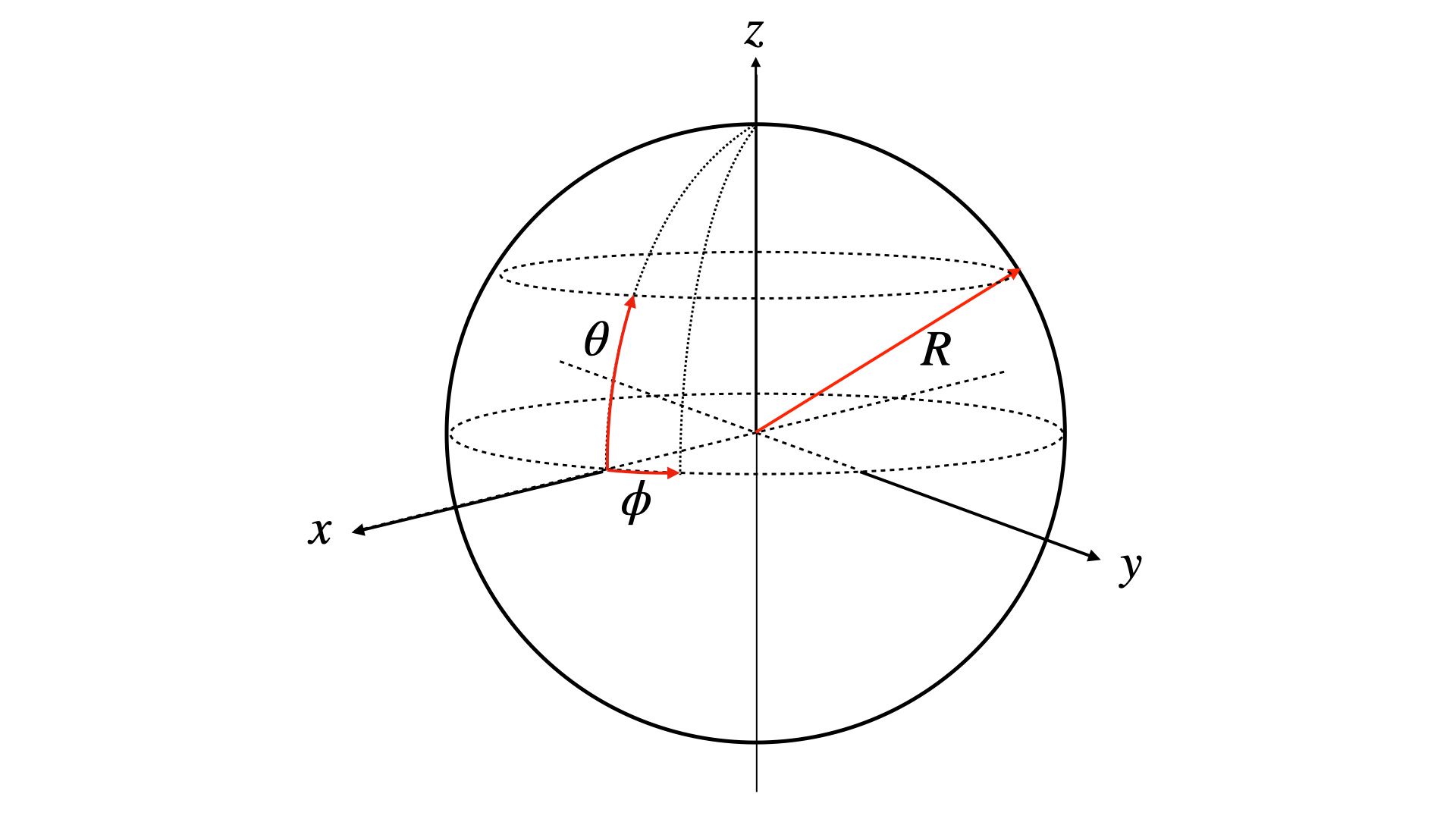
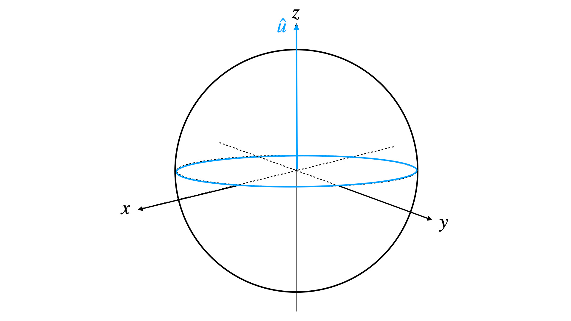
Our goal here is to find the equation of an arbitrary Great Circle on the sphere. This would be a circle on the surface whose circumference is 2𝜋R, which is the largest possible circle that can be drawn on the surface. The center of such a circle is always at the center of the sphere. One specific Great Circle that we can all agree on is the equator. Let’s define a unit vector that is perpendicular to the plane that contains the equator — it is in the direction 𝑢̂ = (𝑢𝑥,𝑢𝑦,𝑢𝑧) = (0,0,1).
Next, suppose we rotate this circle by an angle 𝛾 about the 𝑦-axis, which, of course, maintains the size of the circle on the sphere. This amounts to rotating the unit vector 𝑢̂ away from the 𝑧-axis toward the 𝑥-axis, as shown below.
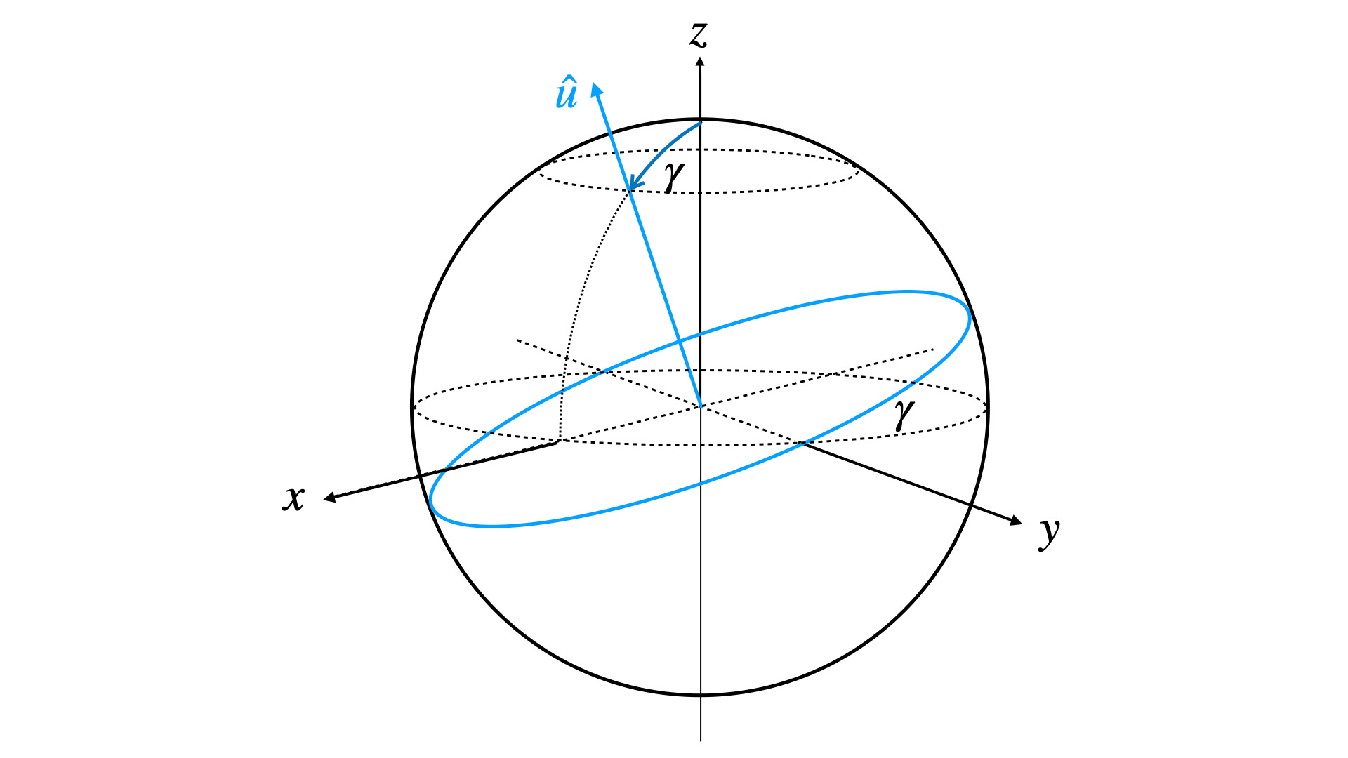
Note how the Great Circle will have extrema in its latitude of 𝜃𝑚𝑎𝑥 = 𝛾 and 𝜃𝑚in = -𝛾, which occur above/below the x-axis.
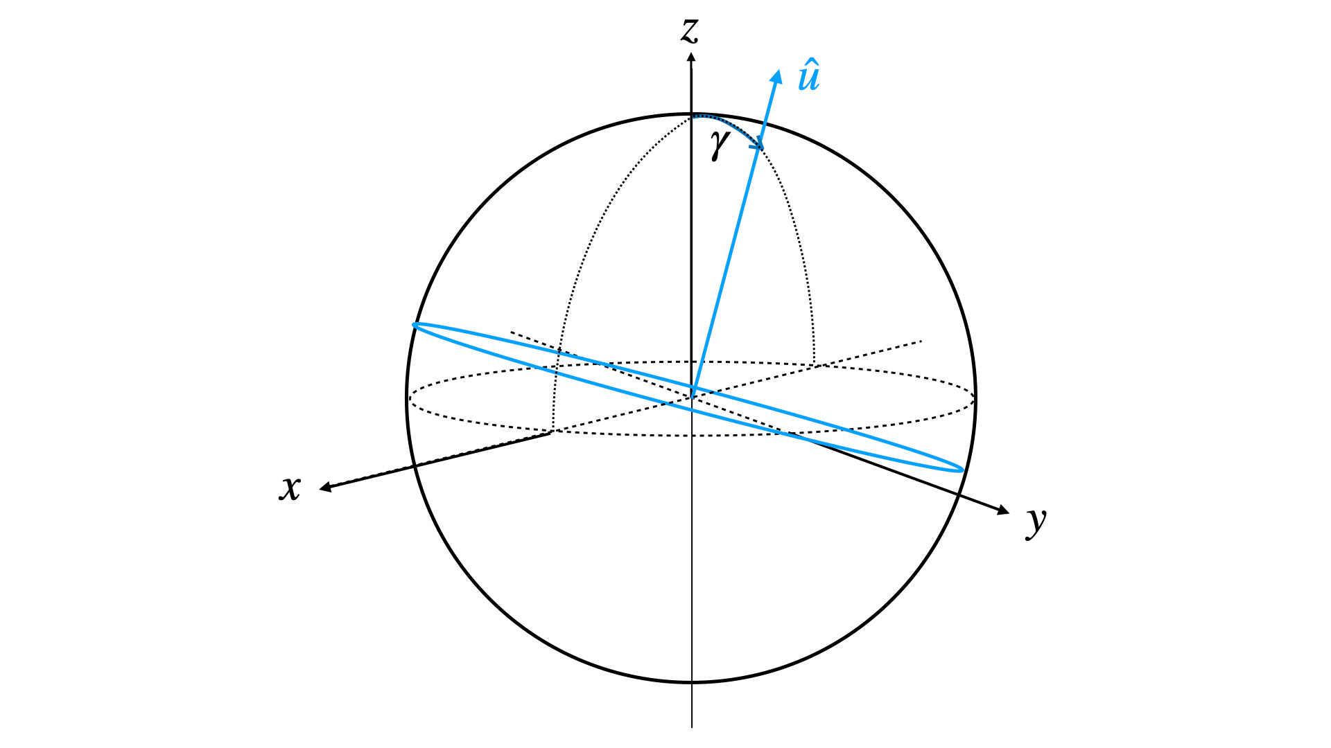
When rotating our equator into a new Great Circle, it might be nicer in the long run if the values of 𝑥, 𝑦, and 𝑧 started out positive for small angles of 𝜃 and 𝜙. So, let’s define 𝛾 as “positive” when rotated toward the negative-𝑥 axis, as shown in our next image. In this instance, the unit vector’s components are
We are now in a position to find an actual equation for our Great Circle. For any point (𝑥,𝑦,𝑧) on the circle, we saw that
where the unit vector
is always directed outward from the center of the sphere toward a point (𝜃,𝜙) on the circle. And so we want to find all of the points on the sphere for which 𝑟̂ is always perpendicular to our previously defined unit vector 𝑢̂. This can be done by setting the dot product of these two vectors to be zero. That is,1
That is, to lie on a Great Circle, the latitude values 𝜃 and the longitude values 𝜙 must be related by the above equation, for a circle tipped by an angle 𝛾 = 𝜃𝑚𝑎𝑥 relative to the equator, and where 𝜙 = 0 at the x-axis.
A general Great Circle located anywhere on the sphere can be described by this rotation plus a further rotation about the 𝑧-axis. If we simply let 𝜙0 correspond to the longitude at which the Great Circle passes through its maximum value of latitude, then the general equation for a Great Circle is
This also tells us that values of the two free parameters — 𝛾 and 𝜙0 — are needed to define an arbitrary Great Circle.
Connection to Mercator
We can imagine a navigator having a Mercator map onboard the vessel from which rhumb lines are computed. But how would one illustrate a Great Circle on such a map projection? We saw in an earlier post that the coordinates on the Mercator Map, which today we will call (𝑋,𝑌), are related to the latitude and longitude on the globe, (𝜃,𝜙), through
where, again, 𝑅 is the radius of the earth. The interesting equation that appears above for the coordinate Y is due to the required “stretching” that we described earlier. Neither Mercator nor anyone else knew of the natural logarithm — or any logarithm — yet. But he understood how the stretching needed to be performed to conserve bearing angles and could sum lines of proper stretching along small increments of latitude — basically “infinitesimals” that could approximate what would be found by the calculus many years later.
A Mercator map can be made which has equally spaced values of 𝑋 in the horizontal direction and equally spaced 𝑌 values in the vertical direction. The grid lines, however, are typically drawn in terms of longitude and latitude, as shown in the image below. Here, the grid is laid out in 15-degree increments of 𝜙 (horizontally) and 𝜃 (vertically). Notice how the 𝜙 grid is uniform, while the 𝜃 grid “expands” away from the equator. The horizontal and vertical coordinates on the Mercator map are related to longitude and latitude by
A “rhumb line” would be defined as a straight line on this map, and a “bearing” on the map – an angle 𝛼 measured from “North” – would be given by tan 𝛼 = Δ𝑋/Δ𝑌.
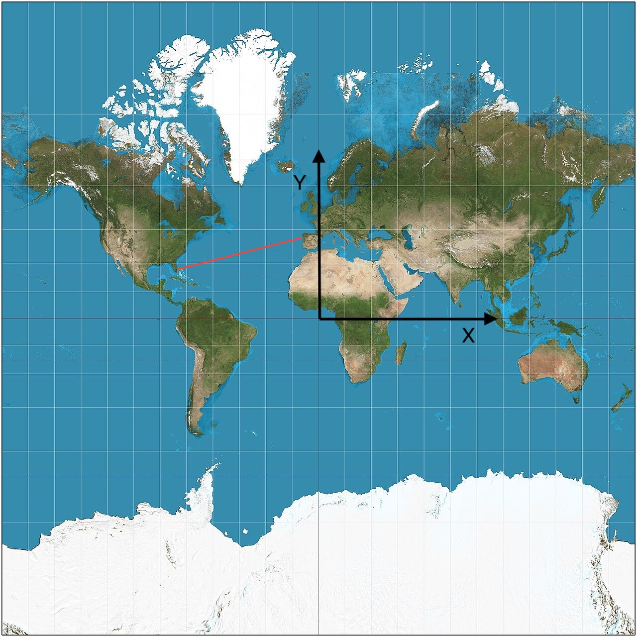
A journey from Florida to Spain could be performed by drawing the appropriate line on the map (in red above), compute the slope m = Δ𝑋/Δ𝑌 and find the bearing angle 𝛼 such that tan 𝛼 = m. Then, one “just” has to maintain that bearing to cross the ocean to one’s destination.
From our discussion in our earlier post on the Hemmi 153 Vector slide rule, and in our Rhumb Line discussion, the special stretching of the lines of latitude can be re-written in terms of the Gudermannian function 𝐺(𝑥),
which yields the following coordinate transformation:
Thus, our equation of a Great Circle,
remembering that 𝛾 = 𝜃𝑚𝑎𝑥, now becomes, in terms of the coordinates 𝑋,𝑌 on a Mercator map,
from which,
since tan[𝐺(𝑥)] = sinh(𝑥), as is used on the Hemmi 153 slide rule.2
The coordinates of a Great Circle drawn on a Mercator map are related through trig and hyperbolic trig functions!
Finally Ready to Compute
Mercator and Gunter are now hugging Gudermann, thanking him for his additional scale, and already eyeing their far-off seats at the bar. Gunter asks the quiet Napier what he thinks now. “This is absolutely wonderful,” says John. “Christoph’s new scale makes calculating the Great Circle a cinch!”
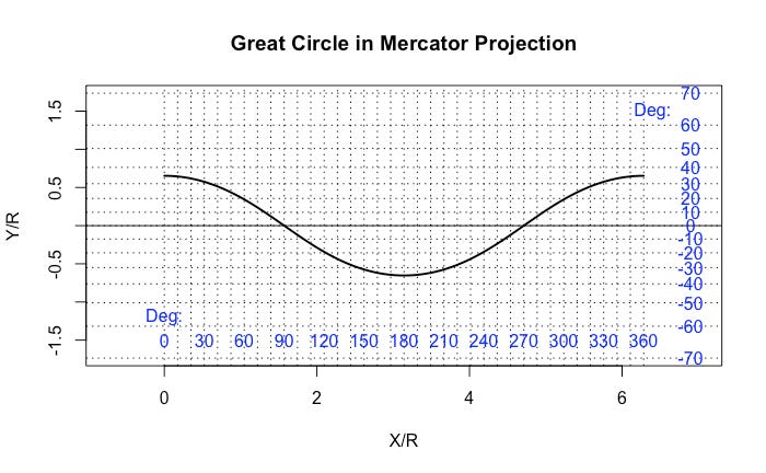
And so, a plot of a Great Circle on a Mercator Map would look something like this:
And our equations above can be mapped out easily by a Vector slide rule. Let’s use the form sinh(Y/R) = tan 𝛾 × cos(X/R). The procedure goes like this:
With 𝛾 provided, for a given 𝜙 = X/R compute tan𝛾 cos𝜙 — then,
find for what value 𝑌/𝑅 does sinh𝑌/𝑅 have that result, using hyperbolic scales on the slide rule.
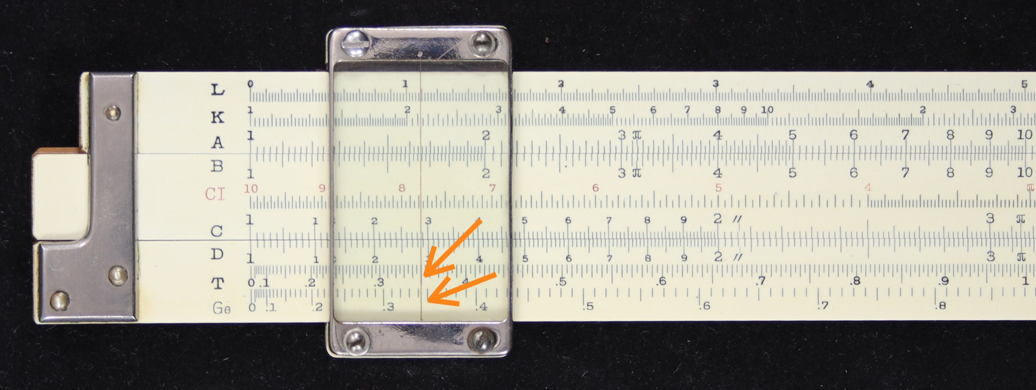
In our image above, I used 𝛾 = 35o. Let’s look at evaluating our Great Circle at X/R = 60o, using the popular Pickett N4. So, we compute tan(35o) ╳ cos(60o) = 0.350 using the S, T, and D scales in the usual way.
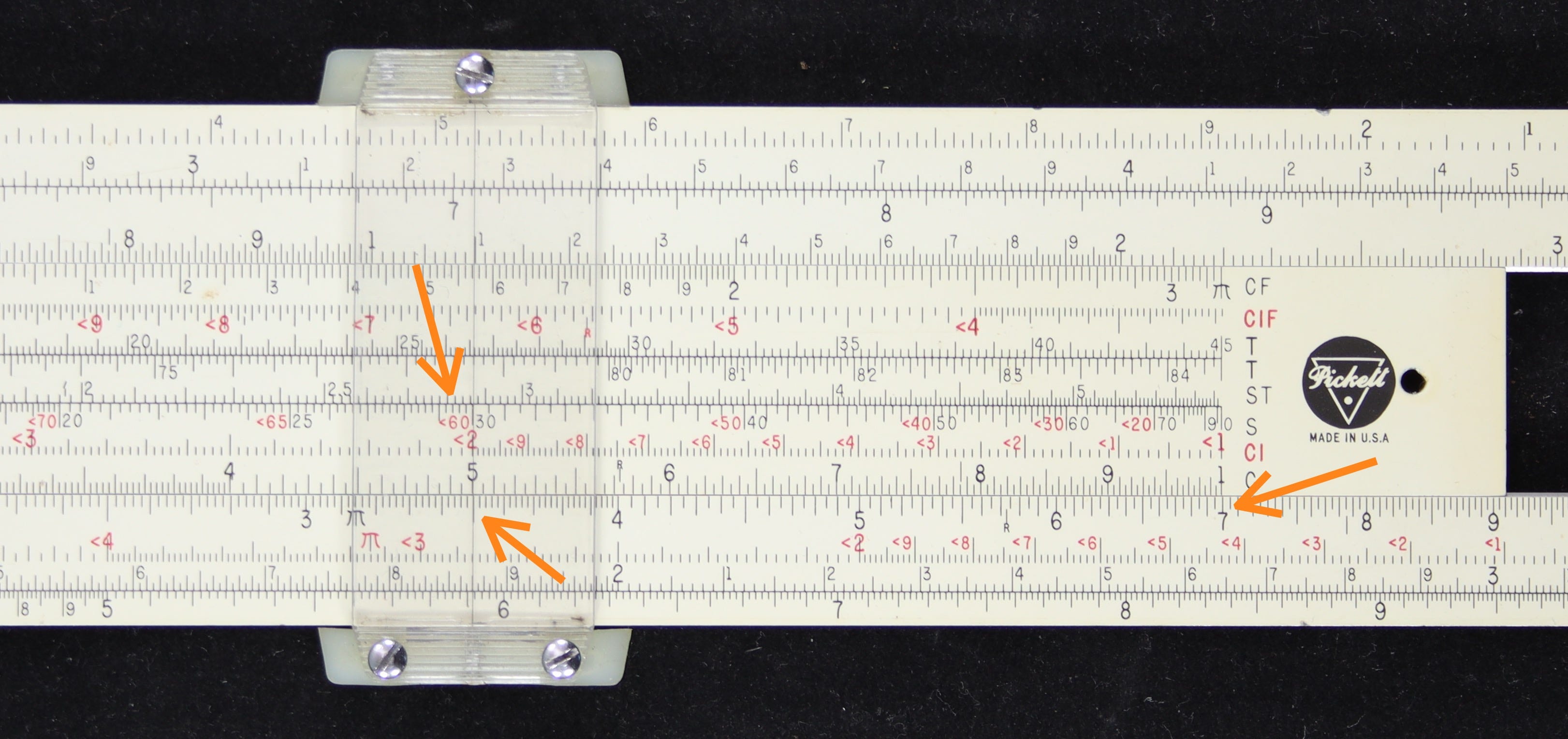
Next, either with the cursor at 0.350 on D and resetting the slide without moving the cursor, or by moving the cursor to find 0.350 on the C scale, we can read off of the SH scale the value of Y/R: 0.342. In other words, sinh(0.342) = 0.350.
This value of Y/R now can be plotted directly on our X/Y map. However, if values of latitude in degrees are marked off on the map and a value of latitude 𝜃 was desired, one would need to use our result to compute 𝜃 = 2tan-1(e0.342) - 𝜋/2, which can be another rather healthy calculation.
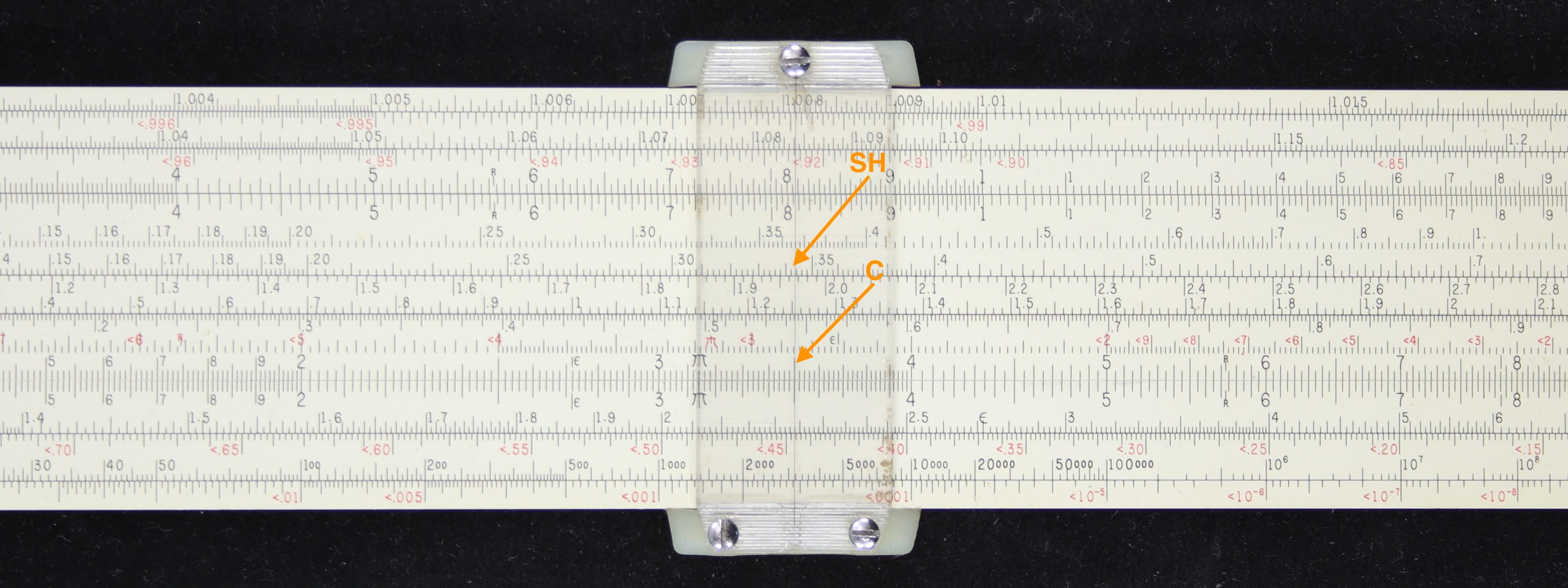
On the other hand, if you happen to have a Hemmi 153 slide rule,
take that “tangent times cosine” result we talked about, and
finding that value on the T scale, read off 𝑌/𝑅 directly on the G𝜃 scale!
And, the angle that gives that value on the G𝜃 scale will be our 𝜃; it can be read directly on the R𝜃 scale in radians, with its value in degrees just above it on the “𝜃” scale!
So, using the Hemmi 153, we compute tan(35o) and cos(60o) separately using the T, and P/Q scales and then compute the product using C and D. We find the result: 0.350 as above. This needs to be our sinh(Y/R) = tan[G(Y/R)]. So, we set the cursor to 0.350 on the T scale. We find directly on the G𝜃 scale a value of 0.342 which, again, is our Y/R. But now, turning the rule over, we can read directly the value of 𝜃 that gives us that value of 0.342 on the G𝜃 scale. We find on R𝜃, 0.336 radians, or, equivalently, on the “𝜃” scale, we find 19.3o. This would be the corresponding latitude on our Great Circle for a longitude of 60o.
The Hemmi 153 scales are perfect for computing great circle coordinates on a Mercator map!3 Now, to get the complete Great Circle, just repeat the process outlined above about 360 times…
Specific Great Circles
Suppose we have two points on the sphere, with coordinates (𝜃1,𝜙1) and (𝜃2,𝜙2), and we want to construct the Great Circle that passes through them. We have two equations with two unknowns that need to be solved simultaneously. In terms of our original Great Circle equation, the following needs to be satisfied:
We know the starting and ending coordinates, but we need to solve for 𝛾 and 𝜙0. This was indeed difficult to do in most cases, and involved much interpolation and iteration in order to get a close approximation of the desired Great Circle. With today’s computers, of course, the solution can be found quickly with numerical techniques.
Suppose, as an example, that we want to travel a Great Circle between points (𝜃, 𝜙) = (5o N, 10oE) and (35oN, 120oE). In the code below we search for the simultaneous roots to our two equations above. The function multiroot() in the R language is designed for just such a calculation.
library(rootSolve)
equations = function(x){  # our input is a "vector" of values (g,p0), each in degrees
   g  = x[1]
   p0 = x[2]
   F1 =  tan(theta[1]/180*pi) - tan(g/180*pi)*cos( (phi[1]-p0)/180*pi )  # = 0
   F2 =  tan(theta[2]/180*pi) - tan(g/180*pi)*cos( (phi[2]-p0)/180*pi )  # = 0
   c(F1,F2)           # = the output of the function is the vector (F1,F2)
}
result = multiroot(f = equations, start = c(g = 45/180*pi, p0 = 45/180*pi))
roots  = as.numeric(result$root %% 360)
g  = roots[1]    # resulting value of "gamma" = "theta_max"
p0 = roots[2]    # resulting value of "phi_0"
Running the above code, we get for our answer:
g= 38 degrees = 𝛾 = 𝜃𝑚𝑎𝑥p0= 93.6 degrees = 𝜙0
But now we want this “circle” plotted on a Mercator map so that we can perhaps make out the changes in rhumb direction along the route. A plot of our Great Circle between our two points, as well as the corresponding Rhumb Line between them, are shown in the plot below in Mercator projection. The dark-red dashed lines correspond to our computed values of 𝛾 and 𝜙0 that we just found:
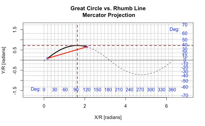
The bearing, or rhumb, must change along the course of a Great Circle. The instantaneous tangential slope at any point (X,Y) along this curve will yield the required bearing at that point.
Since the derivative of sinh is cosh and the derivative of cos is −sin, then the bearing — 𝛼, measured from North — as a function of (𝑋,𝑌) along the path can be found from differentiating our Great Circle equation, namely
which yields
To take our trip along the Great Circle plotted above, a table of the necessary bearings required after every 5 degrees of longitude is produced below, which can be compared to the instantaneous slope of the curve on the Mercator plot above.
##                 1     2     3     4     5     6     7     8
## phi(deg.)   10.00 15.00 20.00 25.00 30.00 35.00 40.00 45.00
## alpha(Deg.) 63.41 64.01 64.92 66.12 67.58 69.25 71.07 72.99
##                 9    10    11    12    13    14    15   16
## phi(deg.)   50.00 55.00 60.00 65.00 70.00 75.00 80.00 85.0
## alpha(Deg.) 74.97 76.94 78.87 80.74 82.52 84.22 85.84 87.4
##                17    18     19     20     21     22     23
## phi(deg.)   90.00 95.00 100.00 105.00 110.00 115.00 120.00
## alpha(Deg.) 88.93 90.43  91.94  93.48  95.07  96.74  98.49
We can see from the table, consistent with our plot, that the original rhumb or bearing needs to be about 63o East of North, and by the time a longitude of about 95o is reached, the bearing should be 90o (or, Due East). Continuing, the ship needs to acquire a bearing of about 98.5o (= 8.5o South of East) by the time the destination is reached. One can see how much easier it would have been to just use the original Rhumb Line between the two points and just maintain a constant bearing.
Final Remarks
A glance at the Mercator projection of a sphere can lead one to believe that the rhumb line is of shorter distance than the Great Circle path. However, this is a distortion created by the expansion of the latitude coordinates on the map. The Great Circle is the shorter route; in fact, the shortest route. In our last example, the rhumb line distance (assuming the sphere in question is the Earth, of radius 𝑅 = 3963 miles) is 7344 miles, while the Great Circle distance is 7141 miles – a savings of 203 miles.4
But it was the ease of implementation of the rhumb line – “just maintain a constant bearing” – that popularized the use of the Mercator projection and transformed the maritime industry. After all, storms, wind conditions, and other factors meant that maintaining any pre-conceived route on a map across an ocean was almost never possible. Great Circle calculations were not straightforward, and having to reproduce them “on the fly” was very daunting no doubt. And knowing when and by how much to change course in order to follow the Great Circle must have been frustratingly difficult. But trying to maintain — and make mid-course corrections to — a constant bearing had to be much simpler for the pilots of sailing vessels in the 1600s.
And, besides, they didn’t yet have hyperbolic scales on their slide rules …

The dot product of two vectors with components (𝑎,𝑏,𝑐) and (𝑒,𝑓,𝑔) is a single number given by 𝑎𝑒+𝑏𝑓+𝑐𝑔. If two vectors are perpendicular to each other, then this product will be zero.
Reminder: sinh 𝑥 = [exp(𝑥) − exp(−𝑥)]/2. In English, the mathematical function “sinh” is most often pronounced by mathematicians as “cinch” or “sinch”. The symbols “sinh(x)” most often would be pronounced, “sinch of ex”.
One might argue that the Flying Fish 1018 slide rule from China is even more efficient. On this rule, the only other known Vector slide rule with the Gudermannian scale, the 𝜃, R𝜃, and G𝜃 scales are all on the same side!
The rhumb path length was computed in our earlier post, while the Great Circle path length requires some knowledge of spherical geometry. The two results are:
I really enjoyed this one.
Mike, very much enjoyed this article. I am sure there is more math to be mined from other map projections than just Mercator.
For example the projections used to map the celestial sphere include the one dating back to antiquity that was used in the astrolabe and the famous Prague city square clock dating back to the Middle Ages.
Basically the complexity here is integrating calculations based on the sphere with the Mercator projection.
Current practices for long distance flights before computers would use a different map that was available in the flight planning room and transfer the coordinates. I will search for this projection. Great circle routes are essential for over the pole routes but are not used in the over water tracks in the Atlantic.