Going Nonlinear -- Part II

Spiral logarithmic scales for that extra digit.

In our last post we looked at the gains that can be made by creating logarithmic scales along circular paths. To first approximation, a circle with the diameter equal to the length of a linear slide rule will have about three times the path length along its circumference, and hence about three times the accuracy when performing computations. Further gains could be made by dividing the logarithmic scale among several concentric circular scales, which provide a path length s = Nπ(d_f + d_i)/2, where d_i is the diameter of the innermost circle, d_f is the diameter of the outermost circle, and N is the total number of circles used. But we also noted that the logarithmic scale in such a situation needs to be laid out according to the angle through each circle, rather than just along the segmented path lengths, as it is the angles that are added when using the circular slide rule.

---

Spiral Logarithmic Scales

Rather than having individual segments made of pure circles, one can create a continuous spiral pattern on the face of the slide rule. A spiral is a curve in which the distance from the origin advances proportional to the angle of rotation. A pure spiral curve with an appropriate logarithmic scaling can provide a long path length for high precision computations.

A spiral curve that begins at the origin, x = y = 0 and with its initial radius (of value zero!) pointed upward. The radius increases at a rate of 1 unit per revolution. In the above, the spiral goes through 10 complete revolutions.

We’ve mentioned that one of the earliest known spiral logarithmic scales was produced by Milburne in about 1650. And Cajori also points out that the same Nicholson who created a segmented linear rule also invented in that year (1697) a spiral slide rule that used two connected “wires, or threads” (along the lines of two cursors) that could be either moved independently or moved together, allowing for the addition of logarithms.

Consider a circular slide rule¹ where a multi-turn spiral D scale is located on the rule near its outer perimeter, with a corresponding multi-turn spiral C scale located at smaller radii and on a sliding (i.e., rotating) portion of the device. Using a cursor, one can add and subtract distances along the spirals much like on a linear slide rule, and hence perform multiplication and division, but with a much longer scale than on a standard slide rule or on a simple circular slide rule.

An example of this technique is the RotaRule made by Boykin, which itself is an adaptation of an earlier rule of the same name made by Dempster. The RotaRule has, among many other scales, a “D50” spiral scale and a “C50” spiral scale. The tightly drawn spirals each go through four revolutions on the rule.

One side of the Boykin RotaRule plus a close-up (right) of the regions containing the spiral D50 and C50 scales. A single decade from 1 to 10 is distributed over 4 turns of the spiral. Click on each image to expand.

The RotaRule has a circular disk with an overall diameter of about 5 inches, but the manufacturer claims that its spiral scales give an accuracy equivalent to a standard linear slide rule of length 50 inches. Note that as the RotaRule has rotating discs, with the D50 on the stationary “stock” and the C50 on a rotating inner disk, then the two scales actually have different path lengths. We’ll take a closer look at both of these scales in just a bit.

Another, more conventional spiral design creates a single curve that takes up most of the face of a circular slide rule. Then, two cursors that can be locked together are used to “measure” the distance (angle) of a single logarithm and, by rotating the pair together, add it to the distance (angle) of another logarithm to perform a multiplication. In this way, the single curve can be of extremely long path length. A very good example is the Gilson Atlas slide rule, an example of which is shown here:

The Atlas Calculator, made by Gilson. This specimen is from 1931.

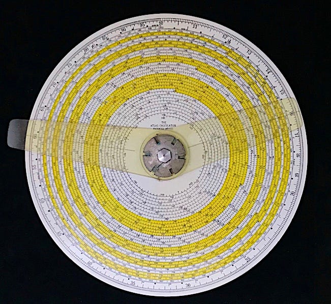
The face of this Atlas slide rule contains a single logarithmic scale that spirals from a starting diameter of about 2 and 3/8 inches outward to a final diameter of about 7 and 5/8 inches. The number of revolutions of the spiral pattern is 30. There is also a separate circular logarithmic scale around the outer perimeter. Its diameter is about 8 inches. (This in itself is a 25 inch scale!) The outer scale is used to estimate a result of a multiplication or division to, say, 3 digits, thus assisting the user when trying to locate the answer on the spiral scale, on which another digit or so can be read.

Calculation of Spiral Path Length

To get at the actual path length attainable on a general spiral scale, let’s consider a curve that goes through N complete revolutions while going from a radius of r₁ to a final radius of r₂. The equation of a general spiral curve is one where the radius as measured from the origin of the curve increases linearly with angle, expressed here in radians:

\(r = k\times \theta.\)

In terms of the parameters of the spiral, the constant k is given by

\(k = \frac{r_2-r_1}{2\pi N}.\)

At the end of the n-th revolution the angle is 2πn and the radius of the spiral would be

\(r_n = r_1 + k\cdot(2\pi\;n) = r_1 + \frac{r_2-r_1}{ N}\times\; n.\)

If we use polar coordinates (r,𝜃), the path length s can be found by adding up the infinitesimal path lengths given by

\(\begin{eqnarray*} ds^2 &=& dr^2 + (r d\theta)^2\\ &=& [(dr/d\theta)^2 + r^2 ] \;d\theta^2 \\ &=& [k^2 + k^2\theta^2 ] \;d\theta^2 \\ ds &=& k\sqrt{1+\theta^2}\;d\theta. \end{eqnarray*}\)

If we use calculus to sum up all of the little “ds”s to get the total path length after passing through a total angle 𝜃, the result is the following:

\(s = \frac{k}{2} \left[ \theta_2 \sqrt{1+\theta_2^2} - \theta_1 \sqrt{1+\theta_1^2} + \ln\left(\frac{\theta_2 + \sqrt{1+\theta_2^2}}{\theta_1 + \sqrt{1+\theta_1^2}} \right) \right].\)

OK, this might look a little frightening. But we can make a reasonable approximation that makes the analysis a bit easier by noticing that the portion of our spiral that we are going to use does not begin at the origin. It begins at some initial radius. If that radius corresponds to the spiral having already rotated through several revolutions, then our starting value for 𝜃 is already a fairly large number. Remember that there are 2π = 6.283 radians in a circle.

Examples of spiral curves with different starting radii: r₁ = 0, 2, and 4 units, corresponding to different initial angles of 𝜃₁ = 0, 4π, and 8π. In each, the final radius is 10 units and advances by 1 unit each revolution. The number of revolutions of the spiral for each case is N = 10, 8, and 6.

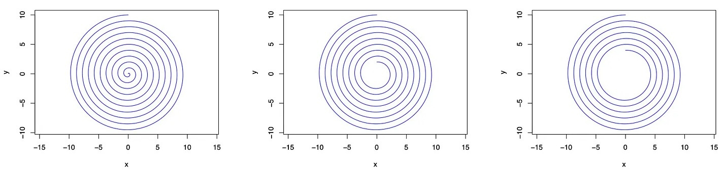
So, starting on a curve that has already rotated many times, the initial angle is already many radians in value. In the figure above, our second case starts after 2 revolutions of a full spiral have already occurred. This means that our starting value for 𝜃 is actually 2×2π ≈ 12 radians. In our third image, the path starts along the spiral curve after 4 initial rotations; thus, the initial 𝜃 is 8π ≈ 24 radians. For such a case, a good approximation for our infinitesimal path length will be ds = k 𝜃 d𝜃 since all of our values of 𝜃² in our analysis will always be much larger than 1. From this we find

\(\begin{eqnarray*} ds &=& k\sqrt{1+\theta^2}\; d\theta \; \approx \; k \;\theta \; d\theta\\ s &\approx& k \int_{\theta_1}^{\theta_2}\theta\; d\theta = k\cdot \frac{1}{2}\theta^2\;|_{\theta_1}^{\theta_2} \\ &=& \frac{k}{2}(\theta_2^2 - \theta_1^2) \\ &=& \frac{k}{2}[(r_2/k)^2 - (r_1/k)^2] \\ &=& \frac{1}{2k}(r_2^2 - r_1^2) \\ &=& \frac{\pi N}{r_2-r_1}(r_2^2 - r_1^2)\\ &=& \pi N(r_2 + r_1) \\ &=& \pi N(d_2 + d_1)/2. \end{eqnarray*}\)

Using this result we can obtain a good approximation of the effective length for our logarithmic scales on the RotaRule and on the Atlas.

Scale Lengths for RotaRule and Atlas

On the RotaRule, the outer scale D50 has an inner diameter of about 4 and 3/8 inches, and an outer diameter of about 5 inches. Thus, the total path length of its four segments would be about π × 4 × (5+4.375)/2 = 59 inches. The C50 scale, however, has inner and outer diameters of 2.25 inches and 3.5 inches. Its total path length is thus π×4×(2.25+3.5)/2 in. ≈ 36 inches. While a claim of “50 inch scales” is certainly true, one could argue that the smaller scale might determine the overall accuracy of calculations performed with the device. But I won’t argue. It’s still 3.5-5 times better than a 10-inch linear slide rule.

The Atlas, being a single spiral scale on the other hand, is easier to interpret. Here, using our approximation formula and the dimensions of the Atlas, we find a total path length of about π×30×(2+3/8+7+5/8)/2 = π×150 in. = 471 inches (39 feet)! Not bad for a rule with a physical diameter of about 8-9 inches.

Like in our discussion of pure circular scales, angles are being added on these types of slide rules, and so the logarithmic scale must be developed in step with the advancement of the angle of rotation. As with our circular case, the ever increasing radius adds more and more circumference. And the logarithmic scale along the path has to be marked according to the advancement of the angle that has been subtended,

\(x = 10^{(\theta-\theta_0)/(2\pi N)},\)

which yields a system by which log x varies proportionally to the angle 𝜃:

\(\log x = \frac{\theta-\theta_0}{2\pi N}\)

At the conclusion of the n-th revolution, the scale would advance to the values shown here:

\(x = 10^{n/N}\)

In code, we would write:²

N = 30
n = c(1:30)
x = 10^(n/N)

which yields the results:

n  1.0000  2.0000  3.0000  4.0000 5.0000   6.0000 
x  1.0798  1.1659  1.2589  1.3594 1.4678   1.5849

n  7.0000  8.0000  9.0000 10.0000 11.0000 12.0000 
x  1.7113  1.8478  1.9953  2.1544  2.3263  2.5119  
 
n 13.0000 14.0000 15.0000 16.0000 17.0000 18.0000
x  2.7123  2.9286  3.1623  3.4145  3.6869  3.9811 

n 19.0000 20.0000 21.0000 22.0000 23.0000 24.0000 
x  4.2987  4.6416  5.0119  5.4117  5.8434  6.3096

n 25.0000 26.0000 27.0000 28.000 29.0000    30
x  6.8129  7.3564  7.9433  8.577  9.2612    10

This is directly compared (and the same, to 5 digits) to a photo of the end points of each revolution on the Atlas scale:

---

You’ll also notice that our path length formulas for concentric circles and for spirals came out the same:

\( s = N\pi (d_2+d_1)/2.\)

But for the case of the spiral, remember that this was an approximation. If the spiral has many turns N and if the final diameter is much larger than the initial diameter, then we are essentially adding up N concentric circles, to good approximation. So it is no real surprise that our estimate for the spiral ends up the same as the result for concentric circles (which, by the way, was exact for equally spaced circles).

In our estimate for the 30-turn Atlas spiral, we found a path length of about 471 inches. For comparison we can compute the path length using the complete formula. The calculation goes something like this:

r1  = (2+3/8)/2; r2 = (7+5/8)/2;  N = 30;  k = (r2-r1)/2/pi/N
th1 = r1/k;  th2 = r2/k
ds  = function(th){ k/2*(th*sqrt(1+th^2) + log(th+sqrt(1+th^2)) ) }
s   = ds(th2) - ds(th1)

Evaluating, I get a value of s = 471.247 inches. Approximation confirmed.

---

Comments on Computational Accuracy

And finally, some words on computational accuracy. We noted in a previous post that the relative error of an answer, dx/x, was inversely proportional to the length of the (linear) logarithmic scale. However, in circular slide rules — either with concentric circles or spiral curves — we actually are adding angles, not path lengths, that are associated with logarithms, according to:

\(\theta = \theta_0 + 2\pi N\cdot \log x\)

for a curve with N turns. As in that earlier post, we can re-write the above in terms of natural logarithms and take the derivative to find that

\(d\theta = \frac{2\pi N}{\ln 10}\;\frac{dx}{x}.\)

So a small error Δ𝜃 in the determination of our final angle yields a relative error Δx/x in our computational result of an amount

\(\frac{\Delta x}{x} = \frac{\ln 10}{2\pi N}\cdot \Delta \theta = \frac{\ln 10}{2\pi N}\cdot \frac{\Delta s}{r}\)

where Δs is the error in marking/reading/setting the cursor along the curve when at a radius r along the spiral. This would imply that the error gets smaller when reading the scale at larger radii. But we must also admit that at smaller radii the numbers on the scale are spaced a bit further apart and so it might in fact be easier to interpolate between tick marks. Hence, the values of “Δs” might be different at different radii as well.

When I look at my Atlas Computer shown above, I find that the tick marks near values of x = 1 are spaced by about 2.5 mm, representing intervals of 0.1 out of 100, or Δx/x of about 0.001. When near x = 10, the spacing is only about 1 mm, representing intervals of 0.1 out of 1000, or Δx/x of about 0.0001. For me (and my eyes), I am able to do a fairly good job of interpolating the 2.5 mm spaces into subdivisions of about 1/10. For the 1 mm spacing, I can maybe do 1/3 -1/4 subdivisions, so say 0.25 mm at best. So, in either case, the factor Δs in the above equation is practically the same — about 0.25 mm. Since the radius goes from about 1.25 inches up to about 3.5 inches, the overall accuracy of the scale does get better at the larger radii by about a factor of three (error goes down by three). My best estimate for the low end (smaller radii):

\(\frac{\Delta x}{x} = \frac{\ln 10}{2\pi(30)} \frac{(0.25~{\rm mm})}{1.25~{\rm in}}\times\frac{1~{\rm in}}{25.4~{\rm mm}} \approx 1\times 10^{-4}. \)

And at the larger radii, this is reduced to about 1/3 × 10^-4 — certainly a bit better, but not an overwhelming factor.

---

Next Time: Helical Logarithmic Scales

Our final example in this series will be that of a three-dimensional curve upon which we may place a logarithmic scale, namely a helix. The situation is illustrated below.

According to Cajori, a design of a helical slide rule was shown in an article in 1842, attributed to a Mr. McFarlane. G. H. Darwin created a helical slide rule design in 1875, and George Fuller created his design in 1879. A variety of other helical slide rules were manufactured by major companies, such as Stanley (London), Otis King (London), Browne (Melbourne) and others. Otis King was perhaps the most popular, and the Fuller Calculating Slide Rule by Stanley was likely the most accurate due to its large effective length. Both of these slide rules were in production for many decades.

And we will examine these two slide rules in further depth in our next post.

An Otis King spiral slide rule.

A Fuller spiral slide rule.

---

---

1. Note that people often call any slide rule with an overall circular layout a “circular slide rule”, even if the scales on the rule itself may not be ideal circles.

2. As usual, we are using the R programming language — R Core Team, R: A Language and Environment for Statistical Computing. Vienna, Austria: R Foundation for Statistical Computing (2025). https://www.R-project.org/.